The overall flow chart of the study is shown in Fig. 1. The details of each step will be introduced one by one later.
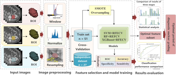
The technical route flow chart of the whole research.
Study patients
This study was approved by the Institutional Ethics Committee of Qilu hospital (Num: KYLL-202205-035-1). Considering that enhanced CT examination is a routine noninvasive technique for suspected patients with ccRCC, the requirement for informed consent was waived. Patients with preoperative enhanced CT scanning and pathologically proven ccRCC between January 2017 and December 2019 were included in the study. The selection criteria for patients are as follows: (a) patients with ccRCC diagnosed by pathology; (b) patients with enhanced CT scans in three periods before surgery; (c) images and clinical data are complete. The patient recruitment flowchart is shown in Fig. 2. In the first four days of data set 1, 76 cases were collected, and 10 cases with incomplete clinical data and 15 cases with incomplete enhanced CT data in three periods were excluded. Finally, we included 51 case studies for training. In addition, we also used the same method to collect 27 cases of data after 2019 as an independent verification set.
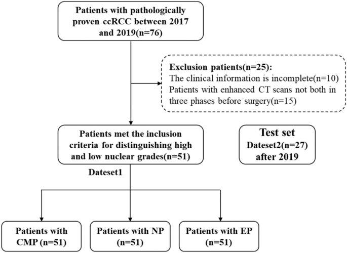
Flowchart of study patients.
CT technique
We employed a SOMATOM Force CT scanner from Siemens Healthcare, located in Erlangen, Germany. Standard protocols were strictly adhered to for all patients. In brief, patients received 60–80 ml of non-ionic contrast agent, iopromide, administered intravenously into the forearm at a rate of 3–5 ml/s using a high-pressure syringe. The scanning protocol included the following phases: Corticomedullary Phase (CMP): The scanning delay time for this phase was set at 20–25 s. During this phase, contrast enhancement within the renal cortex and medulla is maximized, providing detailed imaging of the renal vasculature. Nephrographic Phase (NP): The scanning delay time for this phase was set at 50–60 s. This phase captures the peak enhancement of the renal parenchyma, allowing for visualization of renal structures and pathology. Excretory Phase (EP): Excretory phase scanning was performed 3–5 min after contrast injection. During this phase, contrast material is excreted into the renal collecting system and urinary tract, facilitating the visualization of urinary structures and evaluating for any excretory abnormalities.
Histopathological assessment of nuclear grade
The WHO/ISUP nuclear grades were collected from the histopathological reports at Qilu Hospital of Shandong University. Histopathological evaluations were performed by two genitourinary pathologists with over 10 years of experience in the WHO/ISUP grading system. These grades are determined according to the cytological and nuclear morphological characteristics of renal cell carcinoma. Usually, after histological examination and microscopic observation, the tissue samples of renal cancer are judged according to the cell atypia (cell size, shape, and nuclear characteristics) and the structural characteristics of the tumor (such as the arrangement of tubular structures). Through microscopic observation and histological analysis of tumor tissue, the morphological characteristics of different parts of cells are determined, and the highest grade observed is our label grade. Even so, we think there may still be some deviations, so we divide grades 1 and 2 into low grades and grades 3 and 4 into high grades to form our later experimental data. In addition, because our research only focuses on the best time to distinguish between high-grade and low-grade nuclei, this experimental setup can effectively find the answer, so we designed the whole experiment.
Image preprocessing
Resampling
In this experiment, because different patients may be photographed by different devices, the metadata of some CT images may be different, which may lead to incorrect feature extraction in the later stage. In order to avoid this problem, we first look at the metadata of CT images and find that the pixel spacing of CT images is slightly different. In order to unify the difference in layer thickness and in-plane resolution between images, the B-spline interpolation algorithm is used to uniformly sample all image data to an isotropic voxel size of 1 × 1 × 1 cm. The cubic B-spline interpolation algorithm we adopt is as follows: The pixel value I at the point (({x}{prime},{y}{prime})) is obtained by using the pixel values of 4 × 4 integer points around it,
$$begin{array}{c}Ileft({x}{prime},{y}{prime}right)=sumlimits_{i=0}^{3} sumlimits_{j=0}^{3} Ileft(i,jright)*Wleft(i,jright)end{array}$$
(1)
where (W) is the weight, and its expression is as follows
$$begin{array}{c}Wleft(i,jright)=wleft({d}_{i}right)*wleft({d}_{j}right)end{array}$$
(2)
$$begin{array}{c}{d}_{i}=pleft(i,jright)cdot x-{x}{prime}end{array}$$
(3)
$$begin{array}{c}{d}_{j}=pleft(i,jright)cdot y-{y}{prime}end{array}$$
(4)
$$begin{array}{c}w(d)=left{begin{array}{l}(a+2{)}^{*}mid d{mid }^{3}-(a+3{)}^{*}mid d{mid }^{2}+1hspace{0.25em}hspace{0.25em}hspace{0.25em}hspace{0.25em},mid dmid le 1 {a}^{*}mid d{mid }^{3}-{5}^{*}{a}^{*}mid d{mid }^{2}+{8}^{*}{a}^{*}mid dmid -{4}^{*}ahspace{0.25em}hspace{0.25em}hspace{0.25em}hspace{0.25em},1<mid dmid le 2 0hspace{0.25em}hspace{0.25em}hspace{0.25em}hspace{0.25em},elseend{array}right.end{array}$$
(5)
where the value range of (a) is − 1 to 0, generally a fixed value is − 0.5, and (p(i,j)cdot x) and (p(i,j)cdot y) respectively represent the (x) coordinate and (y) coordinate of the point (p(i,j)), and (d) is an intermediate substitution value. The weight (w) returns to update our initial pixel value to realize cubic B-spline interpolation algorithm.
Window width and level adjustment
Different human tissues or lesions have different CT values. If we want to observe a certain range of tissues, we should choose the appropriate window width and window level, and modifying the window width and window level is usually called the adjustment of contrast brightness. Therefore, improper window width and window level will lead to image blurring and interfere with our feature extraction and image marking of the kidney, so it is necessary to adjust window width and window level for CT images. In this experiment, according to the experience and the gray value of the image in the region of interest, we set the window level to 0 Hu and the window width to 400 Hu by using the SetWindow and SetOutput methods in the IntensityWindowingImageFilter package in SimpleITK.
Artifact correction and image denoising
Especially for images with poor imaging effects, unified artifact correction and image denoising are needed to avoid the extracted features containing a lot of noise. In this experiment, based on the histogram of the image, the distribution difference of pixel values in the image is used to detect the artifact region. In addition, the voxel values are discretized to reduce image noise and improve the calculation efficiency of imaging features.
Pixel value standardization
In addition, in order to speed up the convergence speed of model training, this experiment standardized the image pixel value to make its numerical range between 0 and 1. The formula is as follows:
$$begin{array}{c}norm=frac{{x}_{i}-mathit{min}left(xright)}{mathit{max}left(xright)-mathit{min}left(xright)}end{array}$$
(6)
where ({x}_{i}) represents the value of the image pixel, (mathit{min}left(xright)) and (mathit{max}left(xright)) represent the minimum and maximum values of the image pixel respectively.
Feature normalization
In addition, for the image genomics model, after extracting the image features, the features are also a set of data composed of numbers, similar to image pixels. Therefore, in order to unify the feature dimension and improve the training efficiency of the model, the experiment normalized the features. The processing method is the same as the pixel value standardization method.
Tumor segmentation and feature extraction
All CT images are exported from the Picture Archiving and Communication System (PACS) and then transferred to a separate workstation for manual segmentation using ITKSNAP 3.6 software (www.itk-snap.org). For each tumor, the urologist draws a free 3D region of interest (ROI) on each slice of three -phase enhanced CT. Texture feature extraction was accomplished (with Pyradiomics) on the delineated ROIs in each phase. The 100 candidate features were extracted from each phase based on the original filter, including 18 first-order features, 11 shape features (3D), 3 shape features (2D), 22 Gy level co-occurrence matrix (GLCM) features, 16 Gy level run-length matrix (GLRLM) features, 16 Gy level size zone matrix (GLSZM) features, and 14 Gy level dependence matrix (GLDM) features. See Supplementary Table 1 for the whole feature of extraction. Z-score normalization are used to eliminate the influence between different features.
Data oversampling
From the point of view of the training model, if the number of samples in a certain category is small, then the information provided by this category is too small, and the model will be more inclined to a large number of categories, which is obviously not what we want to see. The high-grade and low-grade data distributions are not balanced in our study, there were 10 cases of low grade and 41 cases of high grade, which would directly result in the model being more capable of learning the majority class (low-grade) than the minority class (high-grade) when training the model. Synthetic minority oversampling technique (SMOTE) is used by us to solve this problem, which changes the data distribution of an imbalanced dataset by adding generated minority class samples, and is one of the popular methods to improve the performance of classification models on imbalanced data23. First, each sample (Xi) is sequentially selected from the minority class samples as the root sample for synthesizing new samples; secondly, according to the up-sampling magnification (n), a sample is randomly selected from (k) ((k) is generally an odd number, such as (k=5)) neighboring samples of the same category of (Xi) as an auxiliary sample for synthesizing a new sample, and repeated (n) times; then linear interpolation is performed between sample (Xi) and each auxiliary sample by the following formula, and finally (n) synthetic samples are generated.
$$begin{array}{c}{x}_{text{new,attr}}={x}_{itext{,attr}}+left({x}_{ijtext{,attr}}-{x}_{itext{,attr}}right)times gamma end{array}$$
(7)
where ( {varvec{x}}_{i} in {{textbf{R}}}^{d} ), ({x}_{itext{,attr}}) is the (attr)-th attribute value of the (i) -th sample in the minority class, (attr={1,2},ldots , d); (gamma ) is a random number between1; (Xij) is the (j)-th neighbor sample of sample (Xi), (j={1,2},ldots ,k); ({x}_{new}) represents a new sample synthesized between (Xij) and (Xi). The characteristic dimension of our sample is 2-dimensional, so each sample can be represented by a point on the 2-dimensional plane. A new sample ({x}_{text{new,attr}}) synthesized by the SMOTE algorithm is equivalent to a point on the connecting line between the point representing the sample ({x}_{itext{,attr}}) and the point representing the sample ({x}_{ijtext{,attr}}). We implemented SMOTE using Python’s sklearn library. Since our dataset is small, the setting of random seeds may cause large differences in oversampling and training results. To address this instability, we chose 30 random The number of seeds, between 0 and 300, and the average result is taken at the end.
Feature selection and model training
We use the wrapping RFECV feature selection method. The feature selection realized by the RFECV method is divided into two parts: the first is the RFE part, that is, recursive feature elimination, which is used to rank the importance of features; the second is the CV part, that is, cross-validation. After feature rating, the best number of features are selected through cross-validation. The specific process we use in this experiment is as follows:
RFE stage
(1) The initial feature set includes all available features. (2) Use the current feature set to model, and then calculate the importance of each feature. (3) Delete the least important feature(s) and update the feature set. (4) Skip to step 2 until the importance rating of all features is completed.
CV stage
(1) According to the importance of features determined in the RFE stage, different numbers of features are selected in turn. (2) Cross-check the selected feature set. (3) Determine the number of features with the highest average score and complete feature selection.
By building SVM24, RF25, and XGB26 classifiers, using five-fold cross-validation to train the model and perform grid parameter optimization in each fold training set, using SMOTE oversampling. The feature weight coefficient of liner SVM and the feature Gini coefficient of RF and XGB are used as the basis for RFECV to filter the feature set. Then the results are averaged by training 30 times with 30 oversampled random seeds, and the average is used to evaluate model performance.
Support vector machine
Given a data set (D={({textbf{x}}_{1},{{text{y}}}_{1}),({textbf{x}}_{2},{{text{y}}}_{2}),ldots ,({textbf{x}}_{{text{n}}},{{text{y}}}_{{text{n}}})}), where ({textbf{x}}_{i}in {mathbb{R}}^{m}) represents the (m)-dimensional feature data, ({y}_{{text{i}}}in {-1,+1}) represents the classification label, and (n) is the total number of samples. Then the optimal hyperplane can be expressed as:
$$begin{array}{c}{{varvec{W}}}^{{text{T}}}x+b=0end{array}$$
(8)
where the column vector ({varvec{W}}={({W}_{1},{W}_{2},dots ,{W}_{m})}^{T}) is the normal vector, which determines the direction of the hyperplane; (b) is the displacement term, which together with the normal vector W determines the distance between the hyperplane and the origin. In order to maximize the classification interval, the objective function is:
$$begin{array}{c}underset{{varvec{W}},b}{{text{min}}} 0.5parallel W{parallel }^{2}+Csumlimits_{i=1}^{n}{xi }_{i}end{array}$$
(9)
$$begin{array}{c}{text{s}}text{.}{text{t}}text{.}{ y}_{i}left({{varvec{W}}}^{{text{T}}}{{varvec{x}}}_{i}+bright)ge 1-{xi }_{i},i={1,2},ldots ,nend{array}$$
(10)
where (C>0) represents the penalty factor, and the larger (C) means the greater penalty for misclassification.
Random forest
When classifying, the RF classifier ({h}_{i}) predicts a label from the set ({c,{c}_{2},dots ,{c}_{n-1},{c}_{n}}) that has been labeled, and expresses the predicted output of ({h}_{i}) on the sample (x) as an N-dimensional vector (({h}_{i}^{1}(x);{h}_{i}^{2}(x);dots {h}_{i}^{N}(x))), where ({h}_{i}^{j}{text{x}}) is the output of ({h}_{i}) on the category label ({c}_{j}), the voting process of RF is publicized as:
$$begin{array}{c}Hleft(xright)={text{arg}}{max}_{C}left(frac{1}{{n}_{text{tree}}}sumlimits_{i=1}^{{n}_{text{tree}}}Ileft(frac{{n}_{hi}, c}{{n}_{hi}}right)right)end{array}$$
(11)
In the formula, ({n}_{text{tree}}) is the number of trees in the RF classifier; (I(*)) is an indicative function; (({n}_{hi},c)) is the classification output of the tree for type ({c}_{j}); ({n}_{hi}) is the number of leaf nodes of the tree. Therefore, RF is a highly generalized integrated learning model.
XGBoost
Assuming that there is a data set containing independent variables (X={{x}_{1},{x}_{2},dots ,{x}_{m}}), classification variables ({y}_{i}) and (n) samples, (K) CART trees are obtained by training them, and the final predicted value (hat{{y}_{i}}) is the accumulation of these tree models value:
$$ begin{array}{*{20}c} {hat{y}_{i} = sumlimits_{{k = 1}}^{K} {f_{k} } left( {x_{i} } right) = sumlimits_{{k = 1}}^{K} {w_{{kq_{k} left( x right)}} } } end{array} $$
(12)
In the formula, (f(x)) represents a CART regression tree, ({w}_{k}) is the leaf weight of the (k)-th regression tree, (q(x)) is the number of the leaf node, that is, the sample (x) will finally fall on a certain leaf node of the tree, its value is ({w}_{q(x)}). XGB adds a regular term (Omega (f)) to the traditional loss function, and uses incremental learning to optimize the function, that is, starting from a constant, each round of training adds a new function on the basis of keeping the previous round of model unchanged, such as the predicted value ({hat{y}}_{i}^{(t)}={hat{y}}_{i}^{(t-1)}+{f}_{t}({x}_{i})) of the (t) -th round, then its loss function (L) is:
$${L}^{left(tright)}=sum_{i=1}^{n}l({y}_{i},{hat{y}}_{i}^{(t-1)}+{f}_{t}({x}_{i}))+Omega ({f}_{t})$$
(13)
where (Omega (f)=gamma T+{2}^{-1}lambda sum_{j=1}^{T}{w}_{j}^{2}), (gamma ) and (uplambda ) are the parameters of the regular term, and (T) represents the number of leaf nodes. XGB can improve the classification accuracy after combining many weak classifiers to form a powerful combined classifier.
Statistical analysis
All statistical analyses were performed using Python (version 3.6.5). The group differences were assessed using a Mann–Whitney U test for continuous variables. The Mann–Whitney U test can be regarded as a substitute for the independent two-sample T test or the corresponding large-sample normal test for the parameter test of the difference between two means. Because the Mann–Whitney U test explicitly considers the rank of each measured value in each sample, it uses more information than a symbolic test. The original hypothesis that (H0) is the distribution of two populations from which two independent samples come has no significant difference. If the probability (p) value is less than or equal to a given significance level (alpha ), the original hypothesis is rejected and the distribution of two populations from which samples come is considered to be significantly different. On the other hand, the original hypothesis is accepted, and there is no significant difference in the distribution of the two populations from which the samples come27,28. In this experiment, a (p) value less than 0.05 indicates a statistically significant difference.
In the classification task, the prediction situation is divided into true positive (TP), true negative (TN), false positive (FP), and false negative (FN). Here, TP denotes the number of cases correctly predicted as positive, FP denotes the number of cases wrongly predicted as positive, TN denotes the number of cases correctly predicted as negative, and FN denotes the number of cases wrongly predicted as negative. The aforementioned four cases can be expressed using a confusion matrix to evaluate the classification performance of the model. Based on the confusion matrix, the proportion of all correct prediction results in the total sample can be calculated using accuracy (ACC) as an evaluation indicator. The higher the index is, the more accurate the model prediction is, and the fewer samples are wrongly predicted.
$$begin{array}{c}ACC=frac{TP+TN}{TP+FN+FP+TN}end{array}$$
(14)
Specificity indicates the sensitivity to negative samples. Essentially, the higher the accuracy rate, the lower the false detection rate.
$$begin{array}{c}SPE=frac{TN}{TN+FP}end{array}$$
(15)
Sensitivity, also known as true positive rate, Recall rate, indicates the proportion of correctly predicted positive samples to actual positive samples, and the higher the sensitivity, the lower the missed detection rate.
$$begin{array}{c}SEN=frac{TP}{TP+FN}end{array}$$
(16)
F1 value (F1-measure) comprehensively indicates the accuracy and sensitivity results. The more proximal the index is to one, the more satisfactory the output result of the model.
$$begin{array}{c}F1=frac{2times TPRtimes PPV}{TPR+PPV}end{array}$$
(17)
The receiver operating characteristic (ROC) curve based on sensitivity and specificity plots TPR on the y-axis and 1 − TNR on the x-axis. The area under the curve (AUC) value, representing the area under the ROC curve, is utilized to evaluate the classification ability of the model. A higher AUC value signifies superior model performance and enhanced classification ability. Finally, through the analysis of the results, we can get the best period of diagnostic nuclear grading.
Ethical approval
The study involving human subjects was reviewed and approved by the Ethics Committee of the Qilu Hospital (No: KYLL-202205-035-1).
Consent statement
All methods were performed in accordance with the relevant guidelines and regulations. All participants gave their written informed consent.
- The Renal Warrior Project. Join Now
- Source: https://www.nature.com/articles/s41598-024-60921-x