Data
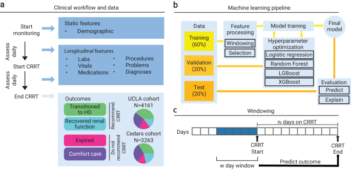
Our dataset consisted of three cohorts of retrospective data of routine clinical processes collected from two different hospital systems (UCLA and Cedars-Sinai Medical Center) with approval and waiver of consent from the Institutional Review Board (IRB) at UCLA (Protocol Number 19-00093). The first cohort was the UCLA: CRRT population (N = 4161 patients), which contained adult patients treated at UCLA that were all placed on CRRT between 2015 and 2021. Adult patients are those that are 21 years of age or older at the start date of treatment. The second was the UCLA: Control population (N = 1562 patients), which contained adult patients treated at UCLA between 2016 and 2021 who were not placed on CRRT. These non-CRRT patients were matched to individuals in the UCLA: CRRT cohort based on race, ethnicity, age, sex, and disease status (via the Charlson Comorbidity Index) via cosine similarity. CRRT patients were already identified prior to receiving the datasets, and therefore no ICD codes were used to categorize patients into the CRRT and UCLA: Control cohorts. The UCLA: Control population consisted of N = 242 (15.5%) patients with known in-hospital mortality. The last cohort was the Cedars: CRRT population (N = 3263 patients), which contained adult patients treated at Cedars who received CRRT between 2016 and 2021.
Our outcome of interest was whether a patient should be placed on CRRT. For the CRRT cohorts at UCLA and Cedars, we constructed the final binary target from four clinical outcomes: recover renal function, transition to hemodialysis (inpatient), comfort care, and expired. The former two represented conditions in which we would recommend CRRT (a positive sample). We recommended CRRT if the patient’s kidneys either completely recovered or the patient was able to stabilize on CRRT and could continue with hemodialysis. The latter two represented conditions in which we would not recommend CRRT (a negative sample). We did not recommend CRRT if the patient did not stabilize on CRRT and continued to end of life care or passed away while on treatment. All patients in the UCLA: Control cohort were not placed on CRRT and therefore did not have CRRT outcome labels. We therefore assigned these patients a negative outcome (to not recommend CRRT) based on the observation that they were not placed on CRRT. There is a possibility that the control cohort with known in-hospital mortality may have benefitted from CRRT, which may have been a source of noise in these assigned outcomes However, there were very few control patients that experienced mortality who consistently had elevated blood creatinine. Therefore, there were few control patients that would potentially fall under a different outcome.
Features describing demographics, vitals, medications, labs, medical problems, and procedures were available for all three cohorts. Demographics were collected once and consisted of information regarding age, sex, race, and ethnicity. Basic descriptive statistics (demographics, outcome variables) for all three cohorts are illustrated in Table 1. The remaining longitudinal features were collected at multiple time points, before and after starting CRRT. The diagnoses and medical problems were documented using ICD-10 codes, along with the respective dates of diagnosis and dates of entry. The procedures were documented using CPT codes and the dates of procedures. Vitals (e.g., temperature, weight, height, systolic/diastolic blood pressure, respiration rate, pulse oximetry, heart rate) were described via numeric value and observation time. Medications were recorded using pharmaceutical subclass identifiers, along with the order date. Lastly, labs were described with the name of the target component or specimen, the value of the result, and the order date.
Data preprocessing
The electronic health record (EHR) data were processed for downstream use in machine-learning pipelines. We defined each sample as a (patient, CRRT session) pair with unique outcomes, as a given individual may have had more than one treatment. For samples in the UCLA: Control cohort, we constructed outcomes and randomly chose a procedure date from the set of procedure dates each patient had undergone to act as a proxy for a treatment start date. For each sample, we loaded and aggregated all longitudinal data over a predefined window of d days. Furthermore, we filtered the training and validation samples to those who were on CRRT for a maximum of seven days. Training a model on patients on CRRT for longer periods of time (eight days or more) made it difficult for the model to learn meaningful relationships between the features before initiating CRRT (which was a pattern we saw with deeper analysis in Methods “Rolling Window Analysis”). These patients were distinct in that their clinical outcomes were temporally far from the clinical data used to train the model to make predictions. Thus, we found that seven days was the optimal time to retain enough patients to train a model and ensure that training data was recent in relation to patient outcome horizons to promote learning. The continuous features over the window were aggregated to the minimum, maximum, mean, standard deviation, skew, and number of measurements. The categorical features over the window were aggregated to the count of occurrences of each category. All ICD codes were converted to Clinical Classifications Software (CCS) codes in order to reduce the number of categories23. All procedure codes were converted to Current Procedural Terminology (CPT) codes24,25. We aligned the names of all vital, all medication, and most lab names across all cohorts in reference to the data contained in the UCLA: CRRT cohort. For vitals and labs, we also unified the units. Additionally, if any values were recorded as ranges bounded on one side, we assumed the value to be the bound (e.g., a value of > 4 was assumed to be 4). We then combined the outcomes, the aggregated longitudinal features, and the static features (patient demographic information). If any feature had a missingness rate of over 95%, we excluded it from our analysis.
We engineered a categorical feature from CCS codes that indicated common reasons for a patient requiring CRRT. Patients were categorized with an indication of heart problems (CCS codes: 96, 97, 100, 101, 102, 103, 104, 105, 106, 107, 108, 109, 114, 115, 116, 117), liver problems (CCS codes: 6, 16, 149, 150, 151, 222), severe infection (CCS codes: 1, 2, 3, 4, 5, 7, 8, 249), or some other disease indication.
These groups, aside from the “other” indication group were not mutually exclusive. Indications for heart problems occurred in N = 3046 (73.2%) of patients in the UCLA: CRRT cohort and N = 2679 (82.1%) in the Cedars: CRRT cohort. Indications for liver problems occurred in N = 3002 (72.1%) of patients in the UCLA: CRRT cohort and N = 1910 (58.5%) in the Cedars: CRRT cohort. Indications for severe infection occurred in N = 2452 (58.9%) of patients in the UCLA: CRRT cohort and N = 2338 (71.7%) in the Cedars: CRRT cohort. Lastly, in the UCLA: CRRT cohort N = 326 (5.7%) patients fell in the “other” category, while 94.3% fell in the former three groups. In the Cedars: CRRT cohort N = 121 (3.7%) fell in the “other” category, while 96.3% fell in the former three groups.
Model training and evaluation
Experiments
We defined an experiment as the full procedure required to train and evaluate a unique predictive model. For each experiment, we specified a cohort or combination of cohorts on which we wanted to train and validate the model. The cohort(s) chosen were divided into train and validation splits using 60/20% of the data, respectively, with the remaining 20% as an internal test split. The entirety of any remaining cohort was used for external testing. As all samples in the UCLA: Control cohort had the same label, the control cohort test data was combined with the test data from the UCLA: CRRT cohort. Otherwise, the label homogeneity would have made it impossible to properly evaluate performance metrics. When training on multiple CRRT cohorts, performance was also evaluated on the isolated samples from each constituent CRRT cohort.
We explored all the following patterns to train and evaluate our methodology: 1) Experiment 1: train on UCLA: CRRT, evaluate on UCLA: CRRT, Cedars: CRRT, UCLA: Control; 2) Experiment 2: train on Cedars: CRRT, evaluate on Cedars: CRRT, UCLA: CRRT, UCLA: Control; 3) Experiment 3: train on UCLA: CRRT combined with Cedars: CRRT, evaluate on CRRT combined with Cedars: CRRT, UCLA: Control; and 4) Experiment 4: train on UCLA: CRRT combined with Cedars: CRRT combined with UCLA: Control, evaluate on CRRT combined with Cedars: CRRT combined with UCLA: Control. Experiments 1-4 were first conducted using the original number of features available in the training split. When training on multiple cohorts (Experiments 3 and 4), the total number of features comprised the union of the features of the individual cohorts. We also re-ran Experiments 1-4 with an extra feature selection step that reduced the feature set to those that existed in all three cohorts. Lastly, we re-ran Experiments 1-3 after reducing the feature set to those that existed in the UCLA: CRRT and Cedars: CRRT cohorts. While the main body of the paper focuses on Experiment 1 (using the original training features) and Experiment 4 (using the features that exist in all three cohorts), results for Experiment 2 (using the original training features) and Experiment 3 (using the features that exist in the UCLA: CRRT and Cedars: CRRT cohorts) are illustrated in Supplementary Figs. 2, 3, 4, 5, 6, 7, 8.
Model hyperparameters and tuning
Each experiment yielded the optimal model of a grid of hyperparameters. Candidate models m included linear and non-linear models: light gradient-boosting machine (LGBM), extreme gradient-boosted decision tree (XGB), random forest (RF), or logistic regression (LR). Each model type had its own (possibly different) hyperparameters that were also tuned as a part of the same grid. We selected the look-back window size w, or the number of days before each patient’s treatment start date from which to aggregate data, from the options of 1, 2, 3, 4, 5, 6, 7, 10, and 14 days. We utilized simple imputation, which refers to mean imputation on continuous or quantitative features and mode imputation on categorical or qualitative features. Note that the imputation method was trained on the training split. Therefore, if features in the training cohort did not exist in the testing cohort, then entire features may have been imputed in the testing cohort. After imputation, the data were scaled between 0 and 1 using minimum-maximum scaling. We also decided on a feature selection procedure based on the Pearson correlation coefficient between each feature and the target variable. This selection was done by limiting to a particular number of features most correlated to the outcome (k-best, where k ∈ {5, 10,15, 20, 25}) or by using a correlation threshold (ρ, where ρ ∈ [0.01, 0.09] at intervals of 0.005). For a detailed breakdown of these hyperparameters, refer to Supplementary Algorithm 1. We ran t = 400 trials of tuning by randomly sampling from the above hyperparameter grid t times. For each trial tj, we loaded the data from the designated cohorts and divided it into the training, validation, and testing portions. We aggregated these three splits over the look-back window of wj days. The imputation and feature selection procedures were trained only on the training split but applied to all three splits. We trained the selected model mj on the train split and then evaluated its performance on the validation split. We then selected the model with the highest receiver operating characteristic area under the curve (ROCAUC) on the validation dataset and evaluated its performance on the testing dataset. Performance was measured by ROCAUC, PRAUC, Brier score, precision, recall, specificity, and F1 score. Confidence intervals were obtained through 1000 bootstrap iterations of the test split.
The optimal hyperparameters for all experiments after tuning are shown in Supplementary Table 1. Simple imputation and feature selection using a correlation threshold were optimal for all experiments. Supplementary Table 1 also describes the number of raw (before processing) and engineered (after processing) features that were available when using the optimal hyperparameters for each experiment. The feature counts are reported both before and after training. The features available for Experiments 1-4 were 2302, 1287, 2791, and 3220 respectively. When reducing the feature set to the intersection of the features between all three cohorts, the features available for Experiments 1–4 were 503, 556, 514, and 556, respectively. Lastly, when reducing the features to the intersection of the features between the UCLA: CRRT and Cedars: CRRT cohorts, the remaining features available for Experiments 1-3 were 626, 662, and 648 respectively.
Subpopulation analysis
In addition to evaluating on the whole test dataset, we evaluated our model on subgroups of the dataset based on different characteristics. Evaluations in this analysis were performed on the combined set of patients who were on CRRT for up to seven days and more than seven days to reflect the performance of the model in a realistic setting. One set of characteristics included common medical reasons for requiring CRRT (identified via ICD code diagnoses), including heart issues, liver issues, and infection. These are some of the most common conditions in which a patient might be hemodynamically unstable and require CRRT. For a list of codes we use for each indicator, refer to Section “Data Preprocessing”. Note that these groups were not mutually exclusive; for instance, a patient may have had a heart condition and also be suffering from a severe infection. Other characteristics were based on sex, race, ethnicity, and age groups.
Rolling window analysis
Each CRRT patient received treatment for a different number of days, so we may have made predictions on variable outcome horizons from the start of treatment. During that time, these patients were under active care, and their condition may have fluctuated due to their own physiologic processes or because of direct medical intervention. A CRRT patient’s outcome may have also stemmed from events that occurred after they began treatment, meaning we would not be able to capture that data for new patients who had not been on CRRT. If the goal of our model is to predict if a patient should start CRRT, we could not train our model on post-start data which would leak information. Though the dynamic nature of CRRT posed a problem to training the model, we could evaluate our model on future data. We therefore implemented a rolling window analysis (visualized in Fig. 1a), evaluating the model (without retraining) on a set of w day windows that each started a day later from the previous window. By monitoring metrics over each window, we could analyze how the predictions and the performance of the model changed as the data neared the outcome horizon (i.e., end of CRRT). If we observed an improvement in performance as the model was evaluated on data closer to the outcome horizon without retraining, we could infer that: 1) outcomes were influenced by events after they start CRRT; and 2) the model had learned meaningful information, and evaluating on the changing information had led to updated predictions for some patients on later windows. Similar conclusions could be drawn if we observed a decrease in performance as the model was evaluated on data further from the outcome horizon without retraining. We performed the rolling window analysis on patients on CRRT for a maximum of seven days because for patients with far-away outcome horizons, data after but near the start date might have still been uninformative.
Note that the rolling window analysis looked at contiguous days of data at once and evaluated a model trained on data before the start of treatment. This procedure was hence completely unaware of previous days or how measurements changed over time which would be used in an ongoing day-by-day predictive task.
Explainability
It is critical when building machine learning models for clinical tasks that the model is understandable to promote transparency, correctness, and trust. We must understand why a model makes its decision, not just how and where it makes the most errors. To this end, in addition to technical performance metrics, we plotted the feature importance of the model applied to the entire test split via SHAP26. We also plotted feature importance for the subset of TP, FP, TN, and FN instances. Additionally, we visualized the features that contributed the most to error via Mealy. Mealy trains a secondary decision tree classifier to predict if the original model will output an incorrect or correct prediction17.
To establish a deeper understanding of our model, we further evaluated if the model was learning distinctions between patients with incorrectly and correctly predicted outcomes. For each feature, we compared pairs of incorrectly and correctly predicted populations in the confusion matrix (i.e., FN vs. TP, FP vs. TN) and tested if the distributions of that feature were statistically significantly different between the two groups. Effect sizes complement the significant results to provide a measure of strength of difference, and thus highlight the features with values that differ the most between incorrectly classified samples and their correct counterparts. We employed a different statistical test and effect size formula depending on the type of feature. For a detailed breakdown of statistical tests and effect size formulas used, refer to Supplementary Table 3. If we rejected, we reasoned that the model may have been using the feature to incorrectly distinguish the populations due to factors such as confounding, and such features with the largest effect sizes should be considered for additional analyses.
Computational software
We implemented our procedure in Python 3.9.16. We primarily used the NumPy 1.23.027 and pandas 1.5.328 packages for loading and manipulating our datasets. Models were implemented via LightGBM 3.3.529 for an implementation of LGBM, xgboost 1.7.430 for an implementation of XGB, and Scikit-learn 1.2.231 for all other models. We used the Optuna 3.2.032 framework for model tuning and the algorithm for sampling from the hyperparameter grid. Statistical tests were computed using the SciPy 1.10.1 and Scikit-learn 1.2.2 packages. We used SHAP 0.42.0 for generating feature importance and explaining model decision-making on particular samples. Lastly, we used the Mealy 0.2.5 package for visualizing model errors.
Statistical analysis
All statistical analyses were performed using Python 3.9.16 and SciPy 1.10.1. When comparing between-group differences in continuous variables, the Shapiro-Wilk test was first used to test for normality; then, normally distributed data were compared using the Student’s t-test, and non-normally distributed data were compared using the Wilcoxon rank-sum test. Hedges’ G statistic was used to describe the effect size. Binary-categorical variables were compared using Fisher’s exact test, and Cohen’s h was used to describe effect size. Multi-categorical variables were compared using the Chi-squared test, and Cramer’s V was used to describe effect size. All statistical tests were two-sided and evaluated at a significance level of p = 0.05, with the Bonferroni correction for multiple testing.
Reporting summary
Further information on research design is available in the Nature Portfolio Reporting Summary linked to this article.
- The Renal Warrior Project. Join Now
- Source: https://www.nature.com/articles/s41467-024-49763-3